Hopfield Network

A discrete Hopfield network is a collection of binary neurons that are recurrently connected to each other. They are useful in pattern completion tasks: a Hopfield network stores a number of memories (for example, patterns representing letters) and can retrieve these memories from partial patterns. They illustrate the concept of an attractor. Each memory is an attractor and a partial cue for that memory is an initial condition. The system can also be understood as minimizing an energy function; the network’s energy value decreases as it settles into stored patterns.

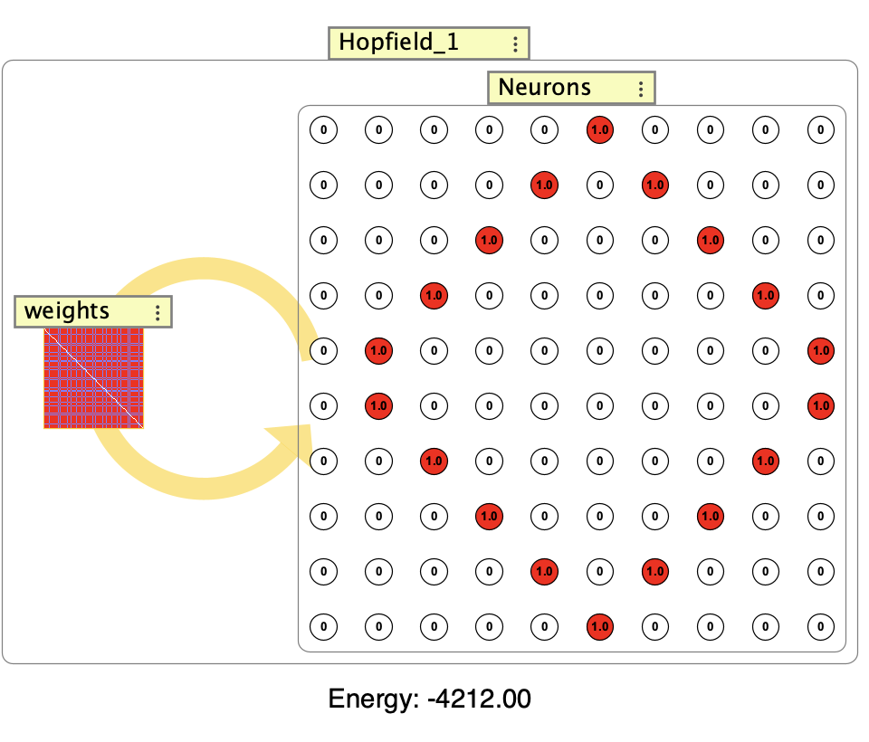
Example Hopfield network showing the neuron grid and weight matrix. The interaction box displays the current energy value of the network.

To get a feel for how Hopfield networks work, try the Hopfield Patterns simulation in the simulations folder (Simulations > Hebb > Hopfield Patterns).

Structure

The Hopfield network consists of:

• A neuron group with binary neurons
• A weight matrix with full recurrent connectivity (no self-connections)
• Training data management for unsupervised learning

The network uses binary patterns (0,1) which are converted to bipolar (-1,1) before Hebbian learning is applied.

Creation / Editing

When creating a Hopfield network, you specify:

• Number of neurons: The number of neurons in the network. Neurons are laid out as a grid by default.

The network is fully interconnected with no self-connections. Hopfield networks have these parameters:

• Update function: Determines how neurons are updated. Three options:
  • Synchronous: All neurons update simultaneously. Does not depend on update order but can produce oscillations.
  • Sequential: Neurons update one at a time in a fixed sequence. More stable than synchronous.
  • Stochastic: A single randomly chosen neuron is updated on each iteration. This is the traditional Hopfield approach and relates to Boltzmann machines.
• Learning rate: Controls how quickly the network learns new patterns when training. In classical Hopfield networks, this is typically set to 1/N where N is the number of patterns to be stored. This normalizes the weight contributions so that the weight matrix becomes the average of the outer products of all training patterns, helping to maintain the network’s theoretical capacity of approximately 0.15 * N patterns for a network with N neurons.

Training

The general training process is covered in Unsupervised Learning. To train a Hopfield network, double-click on the interaction box to open the training dialog.

The network learns patterns using Hebbian learning. Binary patterns (0,1) are converted to bipolar (-1,1) before learning is applied. During training and recall, observe the energy value in the interaction box, which decreases as the network settles into stored patterns.

The training dialog provides a step button to train once through the dataset. Unlike SOM and Competitive networks which benefit from repeated iteration with decaying parameters, Hopfield networks typically use single-pass training where patterns are learned in one iteration.

Training Multiple Patterns

A common workflow for training a Hopfield network is to create a series of patterns and add them to the training dataset before training:

1. Set the network to display a pattern (e.g., by setting neuron activations manually or loading a pattern)
2. Right-click on the network and select Add Current Pattern to Training Data from the context menu
3. Repeat steps 1-2 for each pattern you want to store
4. Once all patterns are added, open the training dialog (double-click the interaction box or use Edit / Train Hopfield from the context menu)
5. In the training dialog, press the Show Matrix Plot button to visualize the correlation matrix of your training patterns

The matrix plot shows pairwise correlations between all training patterns (see Tables for more on matrix plots). Ideally, patterns should have strong correlations along the diagonal (each pattern with itself) and weak correlations off the diagonal. The more correlations appear off-diagonal, the more interference there will be between stored patterns, reducing the network’s ability to reliably retrieve them.

Training Parameters

In classical Hopfield networks, training typically uses a single iteration. The Hebbian learning rule updates all weights once based on the outer product of each pattern with itself. However, you can train for multiple iterations if desired, though this is non-standard.

The learning rate can be set to 1/N where N is the number of patterns to be stored. This normalizes the weight contributions and helps prevent weight saturation. With this learning rate, the weight matrix becomes the average of the outer products of all training patterns. This is the standard formulation in Hopfield network theory and helps maintain the network’s capacity, which is approximately 0.15 * N patterns for a network with N neurons.

Right Click Menu

Common right-click items are described on the subnetwork page.

• Add Current Pattern to Training Data: Add the current pattern to the training dataset.
• Train on current pattern…: Opens a dialog to train the network on the current pattern for a specified number of iterations.
• Train once on current pattern: Train the Hopfield network using the Hebbian rule to learn the current pattern of activity for one iteration. Keyboard shortcut: T
• Edit / Train Hopfield: Opens the training dialog to edit and train the Hopfield network.
• Randomize: Randomize the synaptic weights symmetrically. Keyboard shortcut: R. Uses the Hopfield network’s built-in weight randomizer (configurable in the network’s properties), not the default weight randomizer from network preferences.

Continuous Hopfield Networks

To create a continuous Hopfield network, use a set of Additive neurons in a standard network. These can be connected appropriately and trained by using Hebbian synapses. The user then clamps all neurons, iterates to train the synapses, then clamps all weights. On clamping, see the toolbar documentation.