Restricted Boltzmann Machine
A Restricted Boltzmann Machine (RBM) is an unsupervised learning model that can learn hidden representations of data. RBMs are a type of generative neural network that can model the probability distribution of input data and generate new samples similar to the training data. They consist of two layers: a visible layer (representing the input data) and a hidden layer (representing learned features), with connections only between layers (no connections within a layer).
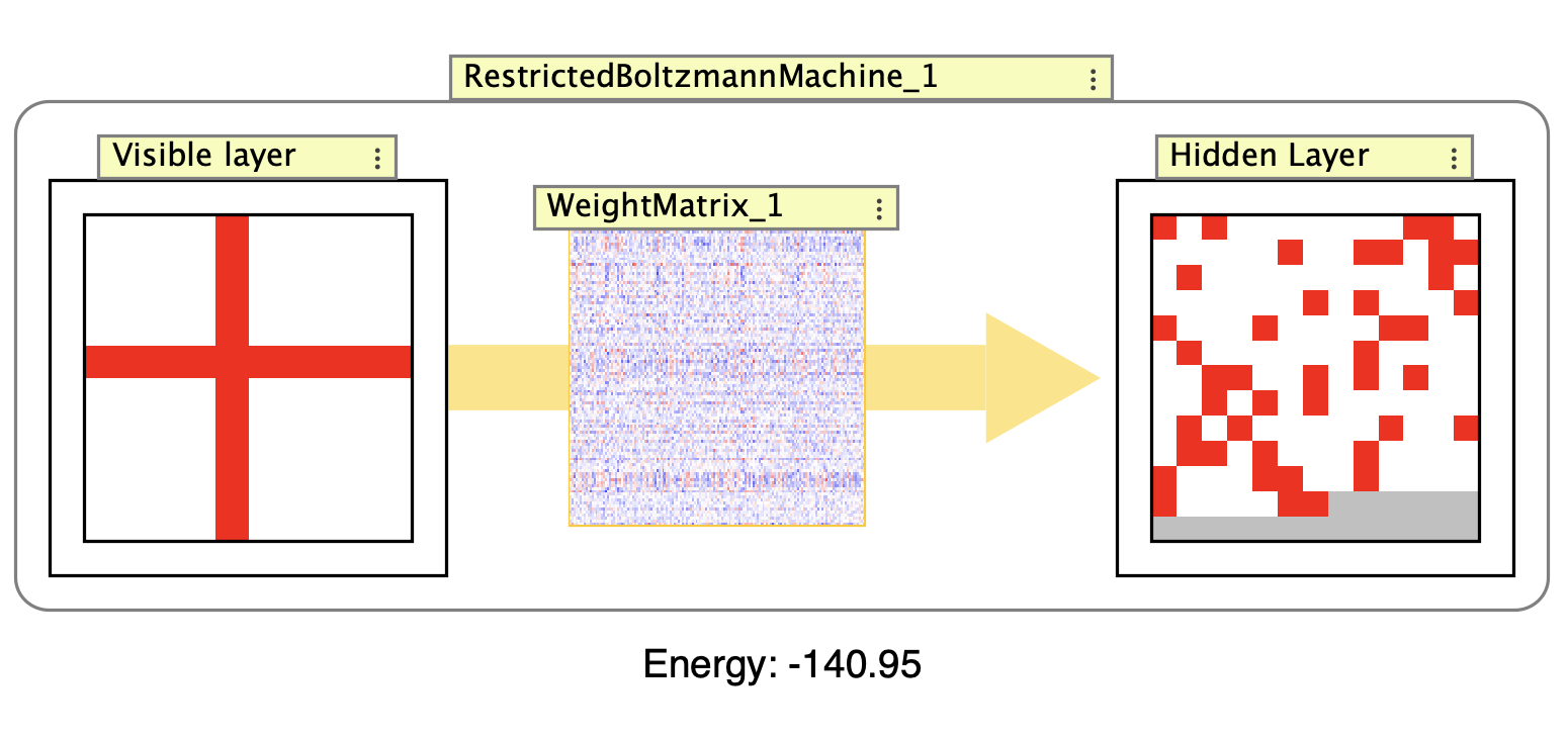
Example RBM showing the visible layer, hidden layer, and weight matrix connecting them. The interaction box displays the current energy value of the network.
RBMs are particularly useful for:
- Feature learning and dimensionality reduction
- Pre-training deep neural networks
- Generative modeling and pattern completion
- Data compression and denoising
The network uses a contrastive divergence algorithm for training, which alternates between positive and negative phases to adjust weights and biases.
To see an RBM in action, try the RBM simulation in the simulations folder (Simulations > Hebb > RBM).
Structure
The RBM consists of:
- A visible layer (input neurons arranged in a grid)
- A hidden layer (feature neurons arranged in a grid)
- A weight matrix with full connectivity between visible and hidden layers (no connections within layers)
- Bias terms for both visible and hidden layers
- Training data management for unsupervised learning
Algorithm
The RBM implements a two-phase learning algorithm based on the energy function:
Energy Function:
\[E = -\sum_i (v_i \cdot \text{bias}_{v_i}) - \sum_j (h_j \cdot \text{bias}_{h_j}) - \sum_i \sum_j (v_i \cdot w_{ij} \cdot h_j)\]where \(v\) are visible units, \(h\) are hidden units, and \(w\) are weights.
Training Process:
-
Positive Phase: Given visible data, compute hidden unit probabilities using sigmoid activation, then sample binary values from these probabilities.
-
Negative Phase: From the sampled hidden states, reconstruct the visible layer and then re-compute hidden states (this gives “reconstructed” or “negative” samples).
- Weight Updates: Update weights and biases based on the difference between positive and negative phases:
Δw = learning_rate * (positive_gradient - negative_gradient) - Sampling: Both visible and hidden units use stochastic binary sampling, where sigmoid outputs are treated as probabilities for setting units to 1 or 0.
Training
RBMs implement the UnsupervisedNetwork interface and can be trained on datasets loaded into the network. The general process is covered in Unsupervised Learning. Double-click the interaction box to open the training dialog.
RBMs use the contrastive divergence algorithm for training. The interaction box displays the current energy state of the network, which should generally decrease during training to indicate convergence.
The training dialog provides a step button to train once through the dataset. Unlike SOM and Competitive networks which use iterative learning with decaying parameters, RBMs typically process the dataset in discrete training passes.
Training Multiple Patterns
A common workflow for training an RBM is to create a series of patterns and add them to the training dataset before training. Since the visible layer is a neuron array, you can use an Image World to create and load patterns:
- Create the RBM network
- Right-click on the visible layer and select
Add coupled image world(this automatically creates and couples an Image World) - Load or create patterns in the Image World (e.g., load images or draw patterns)
- For each pattern you want to train on:
- Display the pattern in the Image World (it will automatically update the visible layer)
- Right-click on the RBM network and select
Add Current Pattern to Training Datafrom the context menu
- Once all patterns are added, open the training dialog (double-click the interaction box or use
Edit / Train RBMfrom the context menu) - In the training dialog, press the
Show Matrix Plotbutton to visualize the correlation matrix of your training patterns
The matrix plot shows pairwise correlations between all training patterns (see Tables for more on matrix plots). Unlike Hopfield networks, RBMs can handle more correlated patterns, but examining the correlation structure can still provide insight into the relationships between your training data.
Training Parameters
RBMs typically require multiple training iterations per pattern. Unlike Hopfield networks which often train with a single iteration, RBMs use iterative gradient descent with contrastive divergence. The number of training iterations depends on the complexity of your patterns and how well you want the network to learn them.
The learning rate controls the step size for weight updates during training. Typical values range from 0.01 to 0.1. A higher learning rate leads to faster learning but may cause instability, while a lower learning rate is more stable but requires more training iterations. The learning rate can be adjusted in the network’s properties or through the training dialog.
Creation / Editing
When creating an RBM, you specify:
-
Number of visible inputs: The number of input neurons, corresponding to the dimensionality of your input data (e.g., 784 for 28x28 pixel images).
-
Number of hidden units neurons: The number of hidden neurons that will learn feature representations. This is typically smaller than the visible layer for compression tasks or larger for feature extraction.
Initial Data
By default, a random dataset is generated for initial training. You can replace this with your own data through the training interface.
Properties and Parameters
- Grid Mode: Both layers are displayed in grid format for better visualization
- Bias Display: Bias values can be shown or hidden in the GUI
- Stochastic Sampling: Units use probabilistic binary activation rather than continuous values
- Randomization: Weights and biases can be randomized using network preferences
- Training Data: Supports loading custom datasets for training
Usage Tips
- Start with a smaller hidden layer for basic feature extraction
- Monitor the energy function - it should generally decrease during training
- The network can be used for pattern completion by setting some visible units and letting the network fill in missing values
- For best results, normalize input data to the range [0,1]
- The stochastic nature means identical inputs may produce slightly different outputs
Right Click Menu
Common right-click items are described on the subnetwork page.
- Add Current Pattern to Training Data: Add the current visible layer activations to the training dataset.
- Train on current pattern…: Opens a dialog to train the RBM on the current visible layer activations for a specified number of iterations.
- Train once on current pattern: Train the RBM on the current visible layer activations for one iteration. Keyboard shortcut:
T - Edit / Train RBM: Opens the training dialog to edit and train the RBM.
- Randomize: Randomize weights, biases, and neuron activations. Keyboard shortcut:
R. Uses the RBM’s built-in randomizers (configurable in the network’s properties), not the default randomizers from network preferences.