Classifiers in Simbrain

The classifier object is a Simbrain front end to a machine learning library, Smile that allows standard machine learning tools to be interfaced with other Simbrain components. It uses ideas and concepts from the Simbrain GUI to make it easy to use these components. However, these are not neural network implementations.

To get a feel for classifiers see the simulations in simulations > machine learning

Three types of classifier are supported: Support Vector Machines, Logistic Regression, and K Nearest Neighbors.

Each classifier is trained on a set of input-target pairs, where the inputs are feature vectors and targets are sets of class labels. The classifier can then be used to assign class labels to new input patterns. Each class label is associated with one of the output neurons. Usually only one output is active for any input (one-hot, winner-take-all).

The classifier is implemented as a subnetwork, with:

• An input layer, consisting of a set neurons. Input vectors are sometimes called “feature vectors” in machine learning.
• An output layer, with one neuron for each possible class.

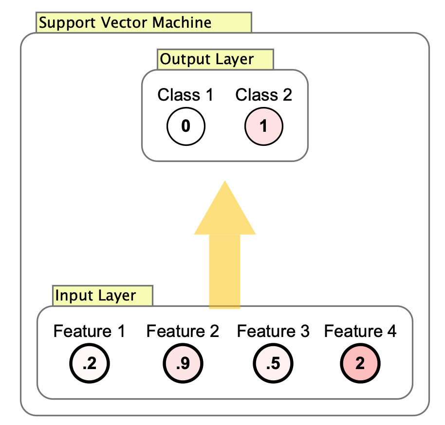
Note that the arrow between the input and output layer cannot be clicked on, which is different from weight matrices and synapse groups, which allow weights to be edited. In the image above note that there is no interaction box on the arrow from the input to the output layer. Machine learning algorithms like these don’t use weights directly, but apply mathematical and statistical techniques directly.

Classifiers are first-class components of Simbrain that can interact with other Simbrain components. Because inputs and outputs are just neuron groups, classifiers can be connected to other Simbrain components. For example, the output of a neural network can be passed into a classifier, and its result sent to another network.

Training and Testing

Double clicking on a classifier’s interaction box opens the training dialog, which provides comprehensive training and testing functionality.

Training Dialog Interface

The training dialog includes:

• Classifier Properties: Configuration panel for algorithm-specific parameters
• Training Statistics: Real-time display of training performance metrics
• Testing Statistics: Performance metrics on held-out testing data
• Training Data Panel: Table view of input features and target classes
• Testing Data Panel: Table view of testing dataset

Data Management

Training and testing data are displayed in interactive tables:

• Input Data: Feature vectors shown as rows in the input table
• Target Data: Class labels displayed with appropriate randomizers
• Class Naming: Uses integer coding internally. Output neurons are labeled “Class 1”, “Class 2”, etc. by default. To use meaningful class names, edit the labels of the output neurons directly (right-click on a neuron and select Edit > Set label). These custom labels will appear in the visualization plot legend.
• Data Editing: Tables support adding, removing, and modifying training examples

Training Process

To train the classifier:

1. Edit training data in the data tables as needed
2. Adjust classifier parameters in the properties panel
3. Click “Train” to fit the model to the current training data
4. Monitor training and testing statistics for performance

Testing Workflow

Testing can be performed in two ways:

• Step through data: Use the step button to test specific inputs from the testing table
• Live testing: Send data to the input layer and update the workspace to see real-time classification

The classifier can also be tested on new data simply by passing data to the input layer and updating the workspace.

Visualizing the Classifier

Right clicking on the interaction box and selecting Visualize Classifier opens a projection plot that provides visual insight into classifier behavior.

Visualization Plot Features

The visualization plot shows:

• Training Data Points: All training examples plotted and colored by class label
• Class Boundaries: Visual representation of how the classifier separates different classes
• Real-time Testing: New data passed through the classifier appears as new points in the plot
• Legend: Shows class names based on output neuron labels

This visualization provides an intuitive and standard way of understanding how the classifier works and how it partitions the input space.

Plot Update Behavior

The visualization plot has specific update characteristics:

• New points: When the workspace updates and the classifier processes input data, new points are added to the plot showing the current classification
• Existing data: The initial training data points shown in the plot are fixed at creation time
• After retraining: If you retrain the classifier with different data or modify training examples, the existing points in the plot will not update to reflect the new model
• After changing class names: If you change the labels of output neurons, the legend in the existing plot will not update

To see updated training data, new classifications of existing data, or updated class names in the visualization, close the current plot window and select Visualize Classifier again from the right-click menu.

Creation Parameters

• Number of inputs: The dimensionality of the input data (i.e., the number of features per training example)
• Number of outputs: The number of class labels (ignored for SVM, which only supports binary classification)
• Classifier Type: Select between different supported algorithms

Support Vector Machine (SVM)

A support vector machine is a binary classifier (that only ever has two output nodes) that separates data into one of two classes by projecting inputs into a higher dimensional space. The model finds a hypersurface that separates the two kinds of inputs in the higher dimensional space using the largest margin possible, as in this image:

SVM only supports two output classes. Internally, class labels are encoded using a bipolar scheme (-1 and 1).

Parameters

• Polynomial Kernel Degree: The degree of the polynomial kernel used to separate the two classes. When the degree is 1, the surface is linear. Higher degrees allow the model to capture more complex, nonlinear relationships between features, but also risk overfitting.
• Soft margin penalty parameter: A regularization parameter that controls the trade-off between maximizing the margin and correctly classifying training points. Larger values prioritize correct classification (resulting in a smaller margin and potential overfitting), while smaller values allow more misclassifications in order to achieve a larger margin and better generalization.
• Tolerance of convergence test: The stopping criterion for the optimization algorithm. Smaller values lead to more precise convergence but longer training times. Larger values result in faster training but less precise solutions.

Logistic Regression

The logistic regression classifier fits a model that outputs probabilities for each class based on the input features. It uses the statistical technique of maximum likelihood estimation to find the parameters of either a sigmoid or a softmax function, depending on whether the task involves two classes (two output nodes in Simbrain) or more (three or more output nodes in Simbrain). These parameters are optimized so that the predicted outputs match the training labels as closely as possible. This is easiest to visualize in the binary (two-category, two output node) case, where a sigmoid function is fit. For example, in the figure below, the input might be the number of hours studied (this would be a case of just one input node), and the target indicates whether each person passed an exam:

Thus the raw output of logistic regression is a probability distribution, which can be shown in Simbrain, and which can often be useful to look at. The input is classified by selecting the class with the highest predicted probability.

Parameters

• Show probabilities: If enabled, each output neuron displays a probability of class membership (a posterior probability) relative to the current input. Together they form a probability distribution over classes. If disabled only one output is highlighted, corresponding to the highest probability output.

K Nearest Neighbors (KNN)

The KNN Classifier assigns a class label to an input based on the most common label among the \(K\) closest inputs in the training set. The idea is illustrated in this figure. The green dot corresponds to the current input or feature vector. The 3 nearest neighbors are found in the dataset (here \(K=3\)) and the green dot is classified with the triangles since most of the neighbors are triangles.

The method works well for small datasets.

Note that the classifier does not need to be trained, it simply finds nearby points in the training set.

Parameters

• K: The number of nearest neighbors used for classification

Right Click Menu

Common right-click items are described on the subnetwork page.

• Edit / Train Classifier: Opens the training dialog to configure and train the classifier.
• Visualize Classifier: Opens a projection plot showing training data points and classification boundaries.