Decay Functions
Decay functions determine how the influence of an object decreases as the distance from its peak increases. They are typically used in spatial or network-based simulations where entities exert less effect the farther they are from a central point or peak.
Decay functions return a scaling factor between 0 and 1 based on a given distance. This factor can be interpreted as a probability or as a strength multiplier. Each decay function defines a different shape for this falloff.
In Simbrain, decay functions are used in odor world for modeling how smells and sensor detection fade with distance, in distance-based connection strategies for creating spatially-organized network connectivity patterns, and in various simulations.
How Decay Functions Work
All decay functions are symmetric around the peak distance. The function reaches its maximum value (scaled by base multiplier) at the peak distance, then decays symmetrically on both sides until reaching 0 at a distance of dispersion from the peak.
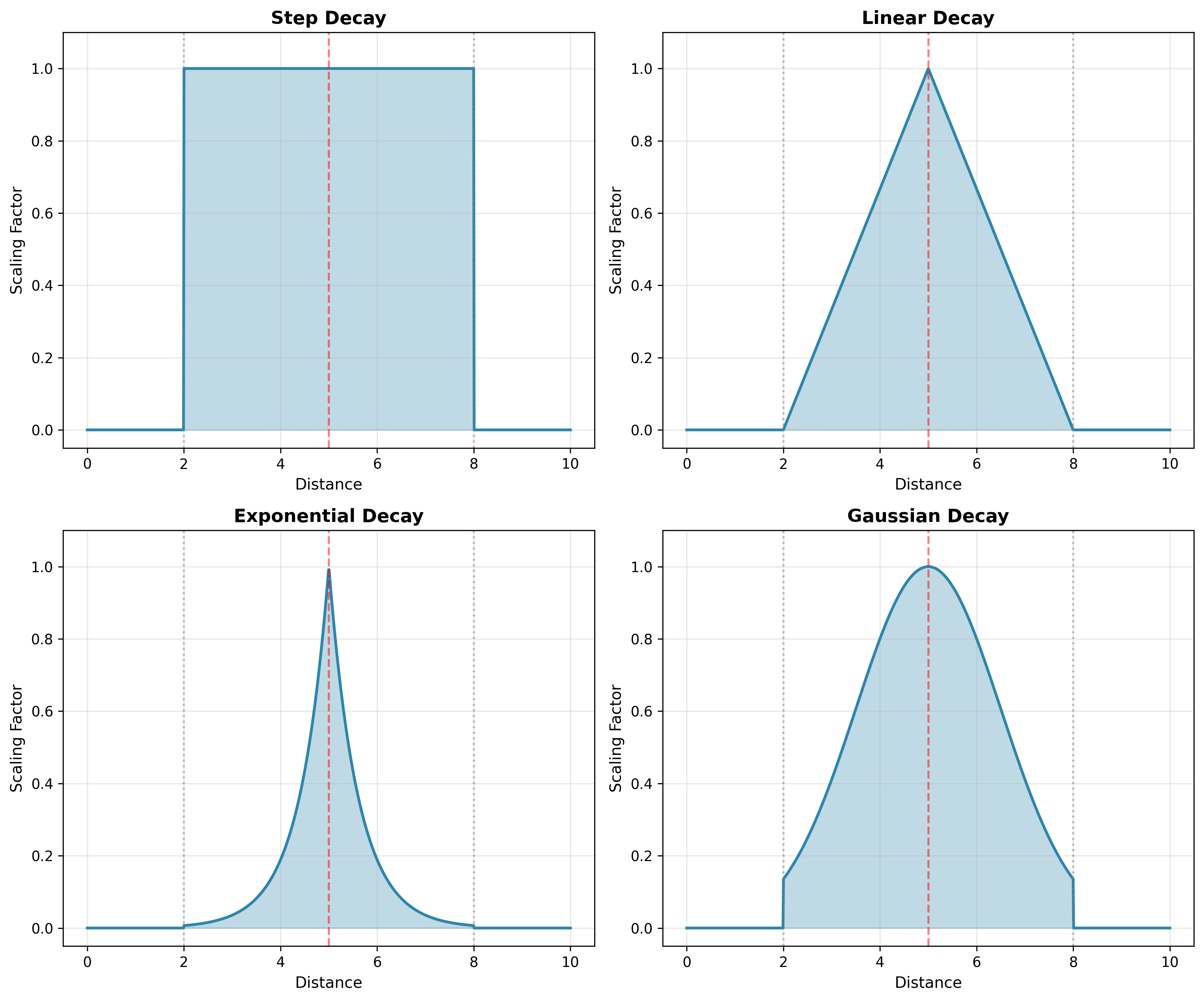
The function evaluates at any distance value (including negative distances, though this does not occur in practice). When peak distance is non-zero, the function creates symmetric shapes centered at the peak: a plateau (step), a triangle (linear), an exponential tent, or a bell curve (Gaussian).
The figure below illustrates the four decay function types with peak distance = 5 and dispersion = 3. However, in most applications peak distance will be 0, meaning the decay simply falls off from the source location according to one of these patterns.
Common Properties
All decay functions in Simbrain share the following parameters:
-
Dispersion: The radius from the peak beyond which the scaling factor becomes zero. Defines the effective range of the decay.
-
Peak Distance: The center of the decay function where it takes its maximal value. The function decays symmetrically on both sides of this point.
-
Base Multiplier: Scales the entire output of the decay function. A value of 1.0 means the peak reaches full strength, while lower values proportionally reduce all outputs. Can be interpreted as a base probability that is further modulated by distance.
Note on Parameterization: All decay functions use dispersion as their primary parameter to provide a consistent interface. Behind the scenes, each function converts dispersion into its natural mathematical parameter (slope for linear, decay rate for exponential, standard deviation for Gaussian). The formulas for these conversions are provided in each function’s description below.
Step Decay Function
The Step Decay function maintains full strength within a radius around the peak, then drops to zero. This makes it useful for modeling binary influence zones where an object either has full effect or no effect at all. The function returns 1.0 for distances within dispersion of the peak distance (i.e., from peakDistance - dispersion to peakDistance + dispersion) and returns 0.0 beyond that range, with no gradual falloff in between. When peak distance equals dispersion, this creates a plateau from 0 to 2 * dispersion.
Linear Decay Function
The Linear Decay function decreases linearly from its peak to zero across the dispersion radius. It is often used when a smooth, predictable drop-off in strength is desired. The function reaches its maximum value at peakDistance, then falls off linearly to 0 at both peakDistance - dispersion and peakDistance + dispersion, creating a triangular shape when peak distance is non-zero. This linear relationship makes it easy to visualize and compute.
For a desired slope m (negative), set dispersion to -1 / m.
Exponential Decay Function
The Exponential Decay exhibits a characteristic exponential falloff pattern, truncated at dispersion. The function reaches its maximum value at peakDistance and decreases exponentially, reaching 0 at both peakDistance - dispersion and peakDistance + dispersion. When peak distance is non-zero, the symmetric exponential decay on both sides creates a tent-like shape with curved sides.
For a desired decay rate lambda, set dispersion to 5.0 / lambda.
Gaussian Decay Function
The Gaussian Decay function models influence using a bell curve, making it ideal for simulating natural falloff patterns such as those found in biology or physics. The function creates a symmetric bell curve centered at peakDistance with smooth, continuous decay within the dispersion range, then truncates to 0 beyond that range.
For a desired standard deviation σ, set dispersion to 2 * σ. At distance peakDistance + dispersion, the scaling factor is approximately 0.135 (13.5% of peak). At distance peakDistance + dispersion/2 (1 standard deviation), the scaling factor is approximately 0.606 (60.6% of peak).