Convolutional Neural Networks
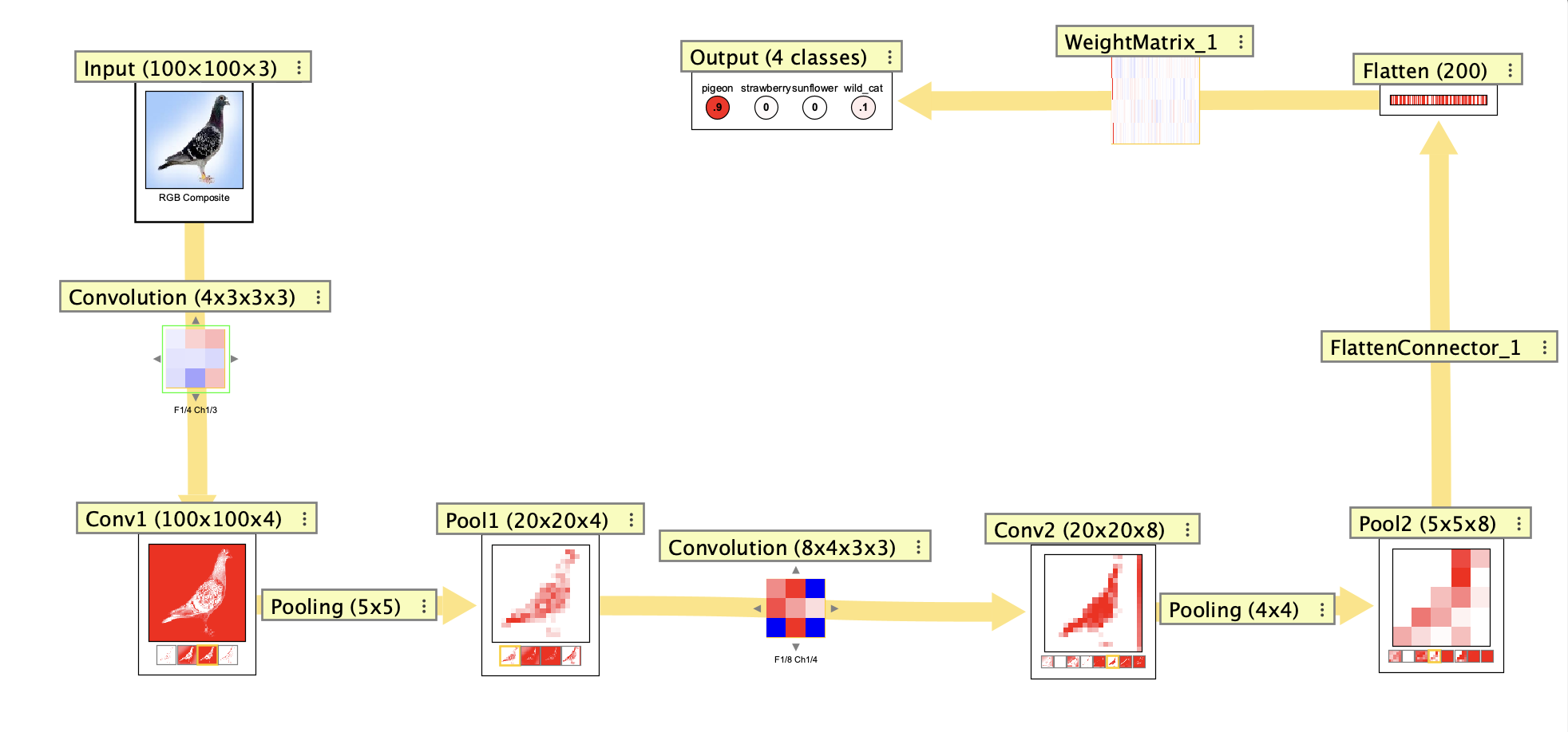
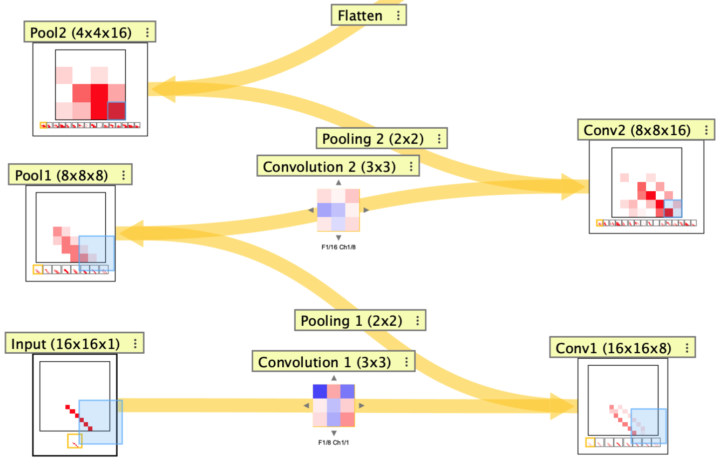
Convolutional neural networks use tensors and spatial connectors to process image-like data. In Simbrain, a CNN is built from TensorLayer nodes connected by convolution and pooling connectors, plus flatten connectors. A ConvolutionalNeuralNetwork subnetwork can wrap the whole pipeline so one network update performs a full forward pass, from image input to class output.
Simbrain’s visual tools make CNNs easier to inspect than they are in many code-only settings. Tensor layers show their spatial shape and channel contents directly, connector dialogs show how stride and padding change those shapes, and the network view makes it possible to watch activity propagate through progressively more abstract feature maps until the final classification layer responds.
You can inspect tensors slice by slice, scroll through filters in a convolution layer, and hover over a pixel to highlight the upstream or downstream patches that influence it. When a CNN is coupled to Image World, you can also step through source images, edit them, and see the effects propagate through the network in real time.
Shape Notation
The main shape-ordering difference to remember is this:
- Tensor layers use
H x W x C, meaning height, width, and channels. Example:28x28x3. - Convolution kernels use
O x I x H x W, meaning output channels, input channels, kernel height, and kernel width. Example:8x3x3x3. - Pooling connectors use
H x Wfor the pooling window size. Example:2x2.
So the main gotcha is that tensor layers use HWC, while convolution kernels use OIHW.
Creating a CNN
There are two ways to build a CNN. The Convolutional Neural Network subnetwork creation dialog steps through the whole architecture in one place: input shape, convolution and pooling stages, dense layers, and output size.
You can also build a CNN outward from an initial tensor layer. Add a tensor layer, right-click it, and use Add Conv Layer..., Add Pool Layer..., or Add Flatten Layer to add the next compatible stage. After flattening to a NeuronArray, continue with outgoing neuron arrays and weight matrices. Neuron arrays can be added to the pipeline in the same way as tensor layers: right-click a tensor layer and use Add Neuron Array to append a dense layer directly. Once the pipeline reaches the desired output NeuronArray, select the input tensor as the source, select the output NeuronArray as the target, and use Create convolutional neural network to wrap the pipeline in a subnetwork.
The tensor-layer list shows each stage and its resulting shape. Convolution and pooling stages let you set properties such as kernel or pool size, stride, padding, activation, and pooling type; see Convolution Kernels and Pooling below for the detailed parameter descriptions.
Tensor Layers
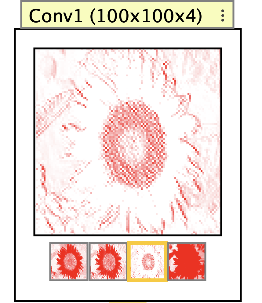
A TensorLayer stores activations in height, width, channel order. Tensor layers are displayed as image-like nodes, with one channel shown in the main view and optional thumbnails for the remaining channels.
Tensor data can be hard to picture because it is organized as a stack of two-dimensional slices rather than as a single grid. Simbrain makes this easier to inspect by showing one channel at a time in the main view, with thumbnails and navigation controls to move through the other slices. Instead of treating a tensor as an abstract 3D block, you can examine it channel by channel as a set of image-like views.
This visualization also makes it easier to interpret receptive field tracing. As you move the cursor over a tensor activation, the trace highlights show how that location connects to downstream or upstream spatial regions, so the tensor’s role in the CNN becomes visible rather than purely symbolic.
The TensorLayer activation functions are part of the tensor/CNN system. They do not reuse ordinary neuron update rules, even when the names are similar. For example, TensorLayer ReLU is separate from the ReLU clipping option described for Linear neurons.
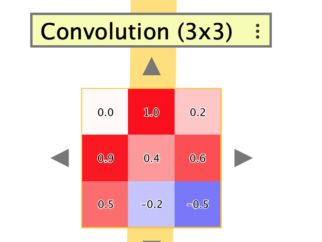
When zoomed in, tensor layers can display numeric activation values as overlays on each cell. This behavior is controlled by the Show numeric overlays preference.
Tensor layers can also be coupled to external components. A single channel can be coupled as a two-dimensional array, and a three-channel tensor can be used as an RGB image source or target.
Tensor-layer interaction boxes append the tensor’s shape using H x W x C notation.
Parameters
- Activation Function: Element-wise function applied after input accumulation.
- Clamped: If selected, incoming inputs are ignored during update.
- Thumbnail Strip: Shows all channels as thumbnails below the main channel image.
- Activations: Current tensor values.
- Biases: Per-element bias values.
Convolution Kernels
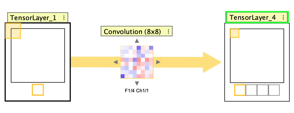
A ConvolutionConnector connects one tensor layer to another using learned kernels. Kernel weights are arranged by filter and input channel. The connector can show either a single kernel at a time or all kernels in a grid.
Convolution is easiest to understand as a small window sliding across the source tensor. The kernel size sets the window size, and the stride sets how far that window moves each time it steps left to right and top to bottom. When stride is smaller than the window, neighboring patches overlap; when it equals the window, they just touch; when it is larger, there are gaps between sampled regions. In Simbrain, receptive field tracing lets you move the cursor across activations and see exactly which source patch contributes to each downstream value.
Padding is mainly used so features near the edges are not underrepresented and so the kernel can still respond to patterns at border locations. Odd-sized kernels are the standard because they have a natural center cell, which makes symmetric padding straightforward. For odd kernels with stride = 1, Same padding adds about (k - 1) / 2 cells on each side, so a 3x3 kernel adds 1, a 5x5 kernel adds 2, and a 7x7 kernel adds 3. Even-sized kernels do not have a single center, so true “same” behavior usually requires different padding on opposite sides. Simbrain currently uses a symmetric approximation, so even kernels still work but can produce unexpected output sizes.
Forward tracing is especially useful here because the highlighted source region makes the effects of stride and padding visible immediately.
The terminology is standard but not especially intuitive. Same is called “same” because when stride = 1, it is often used to preserve the same spatial size from input to output. More generally, it means that border padding is added so edge locations are still included. Valid means no padding is added, so only kernel positions that stay fully inside the original input are used.
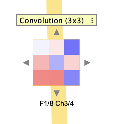
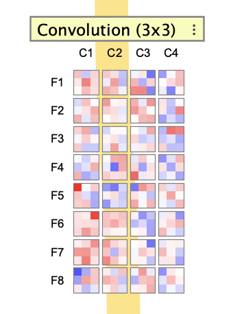
The row labels in the grid correspond to filters, and the column labels correspond to input channels. In single-kernel mode, arrow controls move through filters and channels.
Convolution-connector interaction boxes use the full kernel tensor shape: filters x inputChannels x kernelH x kernelW.
When zoomed in, convolution kernels can display their numeric weight values as overlays, just like tensor activations. This is controlled by the same Show numeric overlays preference.
Parameters
- Kernel Size: Spatial size of each kernel.
- Num Filters: Number of output filters.
- Stride: Step size used when applying the kernel.
- Padding: Valid (unpadded) or Same (padded).
- Increment amount: Amount added or subtracted when changing kernel weights using keyboard controls.
- Kernel Grid: Shows all kernels in a grid instead of one selected filter and channel.
- Kernels: Editable kernel-weight tensor.
Pooling
A PoolingConnector downsamples a tensor layer without learned weights. Pooling preserves the number of channels and changes the spatial dimensions according to the pool size and stride.
Pooling also works by moving a window across the tensor, but instead of applying learned weights it summarizes each visited region. Pool size sets the window size, and stride sets how far that window jumps as it moves across the source tensor. A common pattern is poolSize = stride, which creates non-overlapping downsampling regions. Receptive field tracing helps here too: by moving the cursor across activations, you can see which source region each pooled value came from and how the stride spaces those regions.
In Simbrain, pooling is unpadded, so the pooling window must fit inside the source tensor. This is similar to Valid convolution: if the input dimensions do not divide evenly by the stride and pool size, leftover border rows or columns are dropped. Tracing makes these edge effects easier to understand because the highlight shows exactly where the pooling window can and cannot go.
Pooling-connector interaction boxes use only the pooling-window size, such as 2x2.
The pooling type can be changed dynamically on an existing pooling connector without rebuilding the network.
Parameters
- Pool Size: Spatial size of the pooling window.
- Stride: Step size used when moving the pooling window.
- Pooling Type: Max selects the largest activation in the window. Average averages the window.
Flattening
A FlattenConnector bridges the tensor pipeline to the array-based network system. It copies a tensor’s activations into a NeuronArray, after which ordinary dense layers and WeightMatrix connectors can be used.
Flattening is the point where a CNN pipeline changes from spatial tensor processing to conventional array-based processing.
Receptive Field Tracing
Hovering over tensor activations shows how spatial operations map across layers. This is useful for understanding padding, stride, convolution windows, and pooling windows.
Forward tracing shows the current kernel or pooling-window footprint and the activation it maps to in the next tensor layer. Backward tracing starts from a single activation and shows the source-region footprint that produced it, expanding the receptive field through earlier layers.
When Thumbnail Strip is enabled, clicking a thumbnail selects the tensor channel shown in the main panel. In Kernel Grid View, receptive-field tracing outlines the kernels corresponding to that selected channel. For a source tensor, it highlights a column because that input channel is processed by one kernel from every output filter. For a target tensor, it highlights a row because that output channel is produced by one filter containing one kernel for every input channel. These outlines are available only in Kernel Grid View, and their colors and navigation behavior are controlled by network preferences.
The trace display uses these network preferences:
- Receptive field trace color: Color used for forward trace boxes and connector highlights.
- Backward trace color: Color used for backward trace boxes and connector highlights.
- Receptive field trace mode: Auto Navigate changes the visible channel or filter to the traced one. Highlight Matched shows traces only when the matching channel is already visible. Highlight All shows trace boxes without switching the current view.
Training
Right-click the CNN interaction box and select Train... to open the CNN training dialog. The training dialog provides step, run, stop, randomize, trainer properties, loss display, optional testing metrics, and an error plot.
CNN training uses a separate trainer implementation from Simbrain’s main supervised-learning tools. It follows the same general training concepts described in Supervised Learning and Training Parameters, but updates convolution kernels, tensor biases, and dense weights in the CNN pipeline directly.
- Learning Rate: Learning rate used by Adam updates.
- Beta1: Exponential decay rate for first-moment estimates in Adam.
- Beta2: Exponential decay rate for second-moment estimates in Adam.
- Batch Size: Mini-batch size used for each training iteration.
- Loss Function: Loss used to train the output layer. Options are SSE and Cross Entropy.
- Weight Initialization Strategy: Dense-layer weight initialization strategy.
- Stopping Condition: Optional automatic stopping conditions used while running.
- Test Configuration: Controls periodic evaluation on testing data.
- Compute Accuracy: Computes classification accuracy when targets are one-hot encoded.
When a CNN training dialog creates a default dataset, tensor inputs are initialized with simple synthetic image patterns such as lines, boxes, plus signs, and blobs. Each sample is stored as a flat row sized to the input tensor, but values are placed using the tensor’s height, width, and channel indexing so they map directly to TensorLayer activations; targets are one-hot output vectors. For multi-channel tensors, the pattern is drawn strongly in one primary channel and can be ghosted at lower intensity into the other channels.