How Network Updates Work

When a network is open and the workspace is iterated, an update algorithm is repeatedly called, which is visible in the form of spreading activity in networks nodes and other changes. These changes have a complex logic that is described here. This complexity stems from Simbrain’s effort to support many configurations. This includes networks which mix free neurons and synapses, local learning rules, array-based computations, spiking networks, and more custom forms of update.

The next section gives a broad overview of update focusing on the case of free neurons and synapses. The rest of this document covers more specific topics and forms of update.

Basics

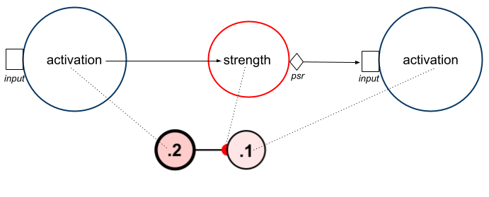
The way information flows from one node to another via a weight provides a useful starting point for understanding how network updates work in Simbrain. In the simplest and easiest-to-understand case, activation in one node is multiplied by a weight strength, and the result is sent to the next node where it becomes the new activation. In the example below assume the weight strength is .5, so that the output is half the input.

There are several variables that play an important role in this process.

• Activation: A number that represents how active a neuron is. The precise interpretation depends on what kind of neuron it is. This is visible as the color of a neuron. More information on the graphical display of activations is in the neuron documentation.

• Strength: How strong or efficacious a synapse is in transmitting information, and whether it is excitatory or inhibitory. More information on the graphical display of strength is in the synapse documentation.

Two additional values are crucial to the process, but are not visible in the GUI:

• Input: Input to a neuron, shown as open rectangles above. A buffer that accumulates inputs from other nodes (via PSRs) and via external couplings. This supports asynchronous or buffered update.

• PSR: Post-synaptic response or “output” of a synapse, shown as diamonds above. Usually the PSR of a node is just source activation times weight. Sometimes the PSR varies over time in response to spikes (see spike responders). The logic of PSR updates is discussed in PSR update below.

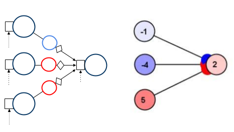
When multiple source nodes connect to a target node, the input to the target node is a summation of PSRs across the source nodes. In the example above, the target node accumulates PSRs from three other nodes. Since in this case there are no spike responders, the target input is a simple weighted sum. In this image we have also shown dotted lines feeding into each input, which emphasizes that information from external couplings can be part of the input to any neuron.

As we will see, all of these values can exist as arrays: activations, inputs, weight strengths, PSRs, etc.

Buffered Update

The default way networks are updated is using buffered update (other options are discussed in update actions). The value of buffered update is that it allows for deterministic updating, that is independent of the order in which network models were added (without this system, you would get different results depending on what order you added items to Simbrain).

Here is the basic algorithm in pseudo code:

for model in networkModels:
    model.accumulateInputs()
for model in networkModels:
    model.update()

The first loop accumulates all the inputs to every network model (mainly neurons, neuron collections, and neuron arrays). These inputs include external inputs from couplings and PSRs from incoming synapses or weight matrices. All of these inputs are added together into an input buffer. The second loop updates all the network models using their update rules, then clears the input buffer in preparation for the next iteration.

Phase 1: Accumulate Inputs

During the accumulate inputs phase, each network model gathers all the information it needs for its next update. For neurons and neuron arrays, this means collecting inputs from incoming connections and external sources into an input buffer.

Each neuron maintains an input buffer that accumulates values from multiple sources: PSRs from all incoming synapses (summed together as weighted inputs), the neuron’s bias value, external inputs from couplings, and any values added by scripts. For neuron arrays, the same concept applies but the input buffer is a vector, with each element accumulating PSRs from incoming weight matrices plus any external inputs.

The PSR (post-synaptic response) mechanism is the key innovation that allows Simbrain to mix connectionist and spiking approaches in a unified framework. Before inputs can be accumulated, the PSR of each incoming connection must be updated. For a single neuron, the accumulate inputs process looks like this:

for synapse in fanIn:
    synapse.updatePSR()
    input += synapse.psr
input += bias

Each incoming synapse updates its PSR value, which is then added to the neuron’s input buffer. How the PSR is computed depends on whether the source neuron is spiking or not.

In the connectionist (non-spiking) case, the PSR is simply the source activation multiplied by the synapse strength:

psr = source.activation * strength

(In rare cases, a neuron update rule may apply a synaptic input modifier to the source activation before multiplication. For example, the Additive (Continuous Hopfield) neuron does this, applying a sigmoidal transfer function to each incoming PSR before they are summed, rather than applying it to the total weighted input, as is typical).

In the spiking case, a spike responder is used to update the PSR. Spike responders allow the PSR to vary over time in response to spikes, creating more biologically realistic synaptic dynamics. When a spike occurs, the spike responder updates the PSR according to its own dynamics (for example, causing it to jump up and then decay exponentially).

Synapses can also have delays. When a delay is set, the PSR value is queued and the actual value used is retrieved from the delay queue.

The same PSR concepts apply to weight matrices connecting to neuron arrays. The PSR matrix is computed by element-wise multiplying each row of the weight matrix by the source activation vector. This factorization of the traditional matrix-vector product (output = weights × input) into two steps allows spike responders to modify individual synaptic responses before they are summed. The target neuron array sums the rows of the PSR matrix to get its input vector. This design means that spiking and non-spiking sources can feed into the same target, with their PSRs (or PSR matrices) simply added together during input accumulation.

Phase 2: Update Models

After all inputs have been accumulated, each network model updates its state. For neurons, this is where the accumulated weighted inputs (which are computed the same way across all neuron types) are transformed into new activations using neuron update rules (which vary widely depending on the type of neuron). For synapses with learning rules, this means updating the synapse strength based on the source and target activations.

The update phase processes models in a specific order to ensure deterministic behavior (see network model update order below). Neurons apply their update rules to transform the accumulated input into a new activation. The update rule has access to the input buffer, the current activation, and any state variables specific to that rule (like a recovery variable for Izhikevich neurons). Synapses with local learning rules update their strengths based on information available to them (typically the source and target activations). These are local learning rules because they only use information available at the synapse itself.

After processing, the input buffer is cleared in preparation for the next iteration.

How Rules Operate on Data

Neurons, synapses, neuron arrays and weight matrices, and spike responders all use a design that separates update rules from the data they operate on. We will start with the case of neurons; the same basic structure applies to other objects as well.

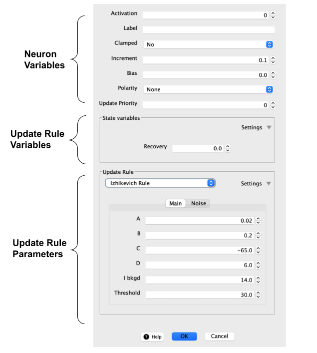
These are the three main types of value associated with a neuron, all of which can be edited using a Simbrain property editor.

First, there are two kinds of data that can dynamically change as a network is updated:

• Neuron variables. These are variables like activation and bias that every neuron has. It also includes the input buffer which accumulates inputs from other network models and from couplings.
• Update rule variables. These are variables associated with the update rule. They are called “state variables” in the property dialog. These variables change as the update rule is changed. In the case shown above, an Izhikevich neuron is associated with a recovery variable.

Then, there are rules which operate on this data:

• Update rules and parameters. These are rule objects associated with a range of parameters that can be edited in property editors. These rules determine how the data are updated. The parameters do not change as the network is updated.

The dialog for the Izhikevich neuron shows where each category is in the dialog.

Data Holders and State Variables

Each update rule creates its own data holder object to store the state variables it needs. For example, the Naka-Rushton neuron rule uses an adaptation variable a, while the Izhikevich rule uses a recovery variable v. When you change the update rule, Simbrain automatically creates the appropriate data holder for that rule.

Data holders serve different purposes for scalar and matrix-based components:

• Scalar data holders store state variables for individual neurons and synapses
• Matrix data holders store arrays of state variables for neuron arrays and weight matrices

Some update rules use simple data holders with minimal state, while others like spiking models require complex state tracking. The data holder appears in the property editor as “State variables” and its contents depend entirely on the selected update rule.

Update Rules can Operate on Array Data

The same update rules that operate on scalar data can operate on array data. For example, in a neuron array, the same categories of data are present: top-level variables like an activation array, and rule-specific variables like a recovery array.

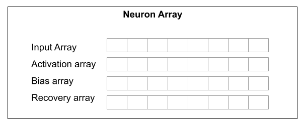
The same rule that operates on scalar state variables with an Izhikevich neuron can operate on arrays with an Izhikevich neuron array. The update rule processes the entire array at once using vectorized operations.

Synapses, Learning Rules, and Spike Responders

These same ideas apply to synapses, but there are now potentially two rule objects. There is a learning rule, which updates the synapse’s strength, and a spike responder, which updates the PSR in response to spikes. Each of these rules can be associated with rule-dependent variables, for example variables which track the course of a spike response (though currently few learning rules or spike responders are associated with special variables).

By default synapses are simple. The learning rule is set to “static synapse rule” and the spike responder is set to “no rule”, in which case the synapse is just a static weight value. But they can become quite complex, with rules modifying weight strengths and spike responses as a simulation runs.

Note that these learning rules are local learning rules that change the weight strength using only information available to the synapse about the source and target neurons it is connected to. A more common way of updating weight strengths is externally, using a trainer.

Weight Matrices

The structure of a synapse is mirrored in weight matrices, but all state variables are now matrices. This is similar to the relationship between neurons and neuron arrays discussed above. Below is a schematic:

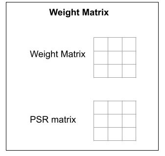
The weight matrix can be updated using a synapse update rule and the PSR matrix can be updated using a spike responder. For a neuron array, the update process iterates through incoming weight matrices, calling updatePSR on each one, then summing the resulting PSR matrices (by adding corresponding rows) to compute the input vector. This allows connectionist and spiking input arrays to feed into the same neuron array.

Update actions

At each network iteration a sequence of actions is executed. Usually only one action is updated, the default update action, buffered update. However, custom actions can be added and update can be customized, either in the GUI, or for even more custom applications, in scripts.

Actions are set using a GUI that is largely the same as in workspace update.

From File > Edit update sequence... the following dialog shows

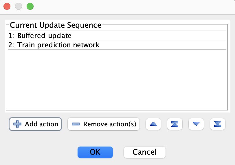
At each network iteration each of these actions is executed in sequence. Some built-in actions can be added from the GUI using the Add action button. Update order can be adjusted using the other buttons or by dragging items on the screen. In this case, the default Buffered update is called followed by a custom action that was created in a script (this is the Simulations > Cognitive Maps > Agent Trails script).

Network Model Update Order

Buffering solves some but not all problems with update order. For example, it makes a difference whether a Hebbian synapse is updated before or after neuron update. Thus, by default, network models are updated in the following determinate order: Neuron, NeuronGroup, NeuronCollection, NeuronArray, Connector, SynapseGroup, Subnetwork, Synapse, All Others.

Note that items within neuron groups and subnetworks are updated in a custom manner specific to the group or network. For example, feedforward networks update the input nodes first, then hidden layers in sequence, then output nodes. To customize even further, custom simulations can be used.

Why Buffering Matters

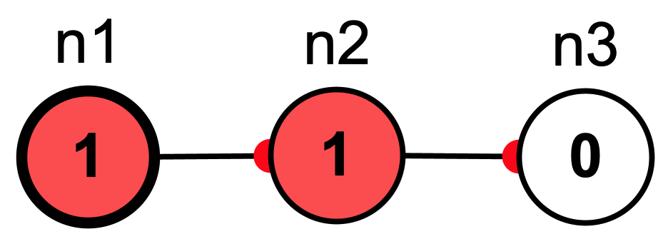
To see why buffering matters, consider the network below. Neuron \(n_1\) is clamped and weight strengths are \(1\). Assume buffering is turned off (in Simbrain this means using priority-based updating, where we specify which nodes are updated in which order).

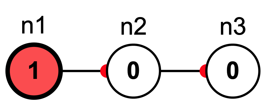
Without buffering, we would get different results depending on update order. If \(n_2\) is updated before \(n_3\) then in the next iteration all nodes will be active:

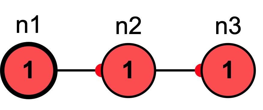
However, if \(n_3\) is updated before \(n_2\) then in the next iteration only \(n_2\) will be active, because when \(n_3\) was updated its input was 0:

Since buffered update accumulates the inputs to every node first and then updates, it does not matter in which order updates occur.

Priority Based Update of Free Neurons

Buffered update is convenient but not always desired. Buffered update makes activation propagate one layer at a time in a layered network, but often we want activations to propagate through all the neurons and layers of a network in one time step. To achieve this we can use priority-based update (in fact, this is how feed-forward works under the hood).

Priority update processes models one at a time in a specific order, allowing each model to immediately affect models updated later in the sequence. Each model accumulates its inputs and updates before the next model processes.

Here is the basic algorithm:

for model in prioritySortedNetworkModels:
    model.accumulateInputs()
    model.update()

Notice that unlike with buffered update, we have a single loop rather than two loops. This means each model makes its new state available to models that update later, enabling sequential processing.

Setting Up Priority Update

To use priority-based update, go to File > Edit update sequence..., remove the “Buffered update” action, and add “Priority update” action. Then set priorities for your network models using the priority table (View > Show priority table...) or the property editor. For example, in a feed-forward network you might set input layer neurons to priority 0, hidden layer neurons to priority 1, and output layer neurons to priority 2.

Setting Priorities

Each network model (neurons, synapses, neuron groups, etc.) has a priority property that determines its update order. Lower numbers have higher priority and are updated first. The default priority is 0 for all models.

The easiest way to view and manage priorities is through the priority table. Go to View > Show priority table... to open the Network Model Priorities dialog:

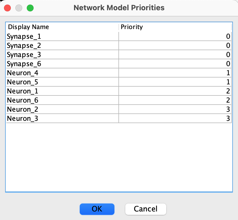
This table shows all network models with their current priorities. You can view all models, edit priorities by clicking on any priority value in the Priority column, sort the table by clicking on column headers, and save changes by clicking OK to apply your priority changes to the network.

Priorities can also be set individually in the property editor for any network model (select the model and press Cmd/Ctrl+E, then edit the “Update Priority” field).

Priority update is useful when you need sequential processing where information flows in one direction through layers. However, in practice, it’s often not needed because relevant subnetworks already update in this way.

Continuous and Discrete Time Update

The network is updated from the workspace or separately using its own run menu.

When the network is updated, a time variable is updated by adding a time-step to it. This updating time can be displayed in two ways, captured by a time-type parameter:

Continuous time: at each iteration time increases by a time step that can be set. Time is displayed in milliseconds. This is used when differential equations are numerically integrated. Generally speaking, the smaller the time-step, the more accurate the numerical integration.

Discrete time: at each iteration time increases by 1. Time is displayed as iterations. In the underlying code the system is still updated by a time-step, but in this mode time is displayed by dividing the continuous time by the time-step.

Consider two neuron models. The first performs a weighted sum on the incoming synaptic connections, puts that value through some function which takes in only that net input as an argument, and produces an output. The second performs a weighted sum as well, but this time the function takes in not only this net input value but also the state (be it the previous net input, activation, or some other value) of the neuron as well. Thus its activation is based not only on its input but its own previous history. In this way we can say that the second neuron has its own internal dynamics. In the first case, the unit of time in the simulation has little importance. The activation does not unfold through time and is only dependent on external input to the neuron, thus the question of granularity is irrelevant. This neuron takes in an input and produces an output in a step by step manner. These two cases can be referred to as temporally discrete or continuous respectively.

Practically speaking even the continuous case is technically discrete as we choose some level of temporal granularity. This is a necessity of simulating temporally continuous situations on a computer which can only consider discrete states. The practice of simulating continuous time on a discrete machine is a major topic in numerical analysis and far beyond the scope of this documentation. The important point is that in complex neuron models with internal states the notion of when things happen and how long they take to happen becomes important, and we simulate that fundamental temporal continuity by choosing typically very small but meaningful and quantified discretized time-steps.

Neuron update rules are associated with a time type. Any time a single continuous update rule is used in a network, time is automatically changed to continuous. This can however be overridden by manually adjusting time type in the network properties. If there is a single continuous neuron or synapse in a simulation, the network panel will display time in seconds. Otherwise time is displayed in iterations.